Authors: Jerome Gammie and Cibele Amaral

Contributors: Natasha Stavros, Ty Tuff, Claire Monteleoni, and Nayani Ilangakoon

We are already seeing the terrifying impact of climate change on our forests, with ever more frequent and ever more severe wildfires. Such events are only part of the impact of climate change – heat, drought, and more could also affect natural ecosystems health. We want to be able to predict the health of a particular piece of forested ecosystem in the future under these changing conditions. We can use digital twins of a section of forest to model how it may look in different scenarios, but we need to be able to compute various metrics of forest health from the digital twin to make meaningful comparisons to present conditions. 

One such metric is Water Use Efficiency, or WUE. This measures the ratio of carbon stored by plants to water evaporated by plants, in grams of carbon stored per kilogram of water evaporated in one day between sunrise and sunset [1]. ECOSTRESS WUE data, which we focused on, is generated at a 70 meter resolution from a large process-based model using an algorithm described here [2]. 

This is where our project begins – we want to be able to generate a WUE value from data that can be easily gathered or simulated from a digital twin. This data includes elevation, slope, and aspect (which should be roughly the same for the digital twin of a region in the future as it is for the region at present), land cover (which is a part of what the digital twin would model and so should be easy to derive), and forest structural data from GEDI waveform lidar (which we believe can be simulated from the twin’s spatial information).

This problem lends itself to an application of machine and deep learning. We have all of the data listed above – elevation, slope, aspect, land cover, lidar metrics, and WUE – from which we can build a dataset with ground truth values to perform supervised learning, also allowing us to bypass process-based models. With enough diversity in the training data, we can expect that the data generated from the digital twin will be reasonably within the domain that the model was trained on, and so we can expect reasonable predictions from the model. 

Returning to the big picture, our ability to predict WUE, or even other important metrics of forest health, is a critical part of being able to use digital twins to understand how our forests will change with time, climate change, and other factors and how those changes will affect ecosystem’s health and productivity.

The datacube challenge
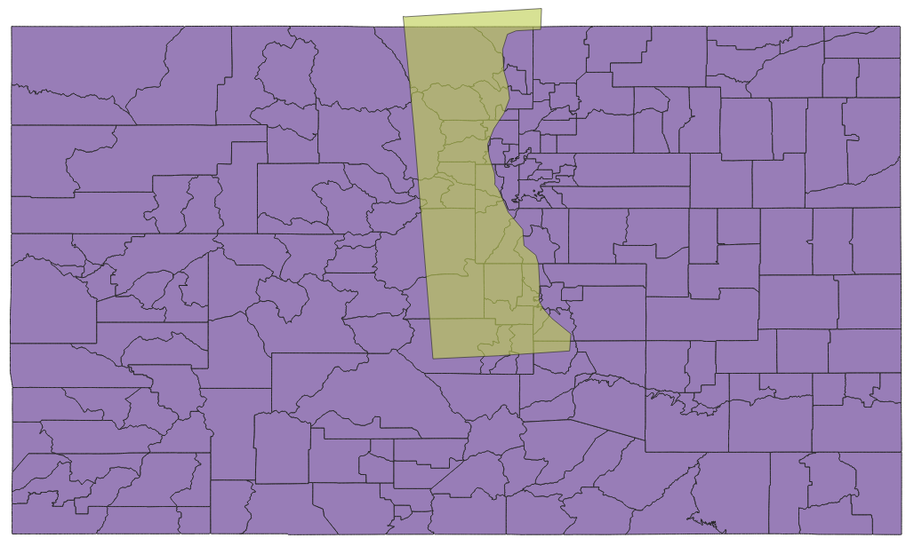
Our model starts with the creation of a harmonized datacube from preprocessed (e.g., masked, composited) remote sensing-based data, such as elevation, aspect, slope (SRTM) [3], land cover (NLCD) [4], forest structural metrics (GEDI L2B) [5] and water use efficiency (ECOSTRESS) [1] collected from our study site: Colorado Front Range

Left: Area of Interest overlaid on a map of Colorado. Center: SRTM data clipped to the area of interest. RIght: NLCD Data clipped to the area of interest.

We wanted to combine the datasets listed above into datacubes  - one cube for each 70m ECOSTRESS WUE value. This presents problems because the elevation, slope, aspect, and landcover data are at 30m resolution, and the GEDI data is at 25m but is not gridded! Even worse, neither 30 nor 25 divide 70 in a nice way. We wanted to retain the spatial character of the data so that we could take advantage of spatial relationships with convolutional models, so we decided to divide each 70m ecostress raster grid square into 5m pixels (the greatest common factor of 70, 30, and 25), creating a 14x14 grid. These turned out to be difficult dimensions to work with so we added a 1 pixel (5m) buffer to each side, borrowing 1 pixel from data that falls within the confines of neighboring ecostress raster grid squares. This created a 16x16, 80m grid centered on the 70m ecostress grid square. We had to resample the raster data and interpolate the GEDI data to determine what values belonged at each pixel in each combined data cube. 

We performed nearest neighbor interpolation on the GEDI data to grid it. We therefore had to find the nearest GEDI centroid to the center of each pixel in every datacube. To do this in an efficient manner, we first initialized a large array the same size as the ECOSTRESS WUE raster array. We then created a list at each index in the array of every GEDI centroid that falls within the corresponding grid square. Then, at each grid square, we could greatly reduce the number of centroids to consider in the interpolation process by starting at that grid square and working outwards in rings of grid squares, building a list of GEDI centroids, until reaching a stopping point.

This process resulted in 16x16 datacubes with 68 channels (4 raster channels, 62 GEDI channels, a channel with the index of the nearest GEDI centroid, and a channel with the distance of the nearest GEDI centroid). The nearest centroid to the center of a datacube may be hundreds of meters away, meaning that the interpolated data could be wildly inaccurate. Saving the shortest distances allowed us to remove samples with distances above some threshold. These channels are then cut out for the training process. The datacubes themselves can be saved as csv or hdf5 files. The first allows for easier manual inspection of the data, while the second greatly improves model training times. 

Visualizations of raster data layers of a single datacube prior harmonization. From left: SRTM, Slope, NLCD, Aspect. Note that while each channel’s data appears to be in 30m blocks, none of the blocks overlap perfectly.

Finally, we partitioned the data into a test set and a number of cross validation folds containing training and validation data. The analysis below is conducted on a randomly sampled subset of the data with one cross validation fold, 100000 samples in the test set, 280000 samples in the training set, and 120000 samples in the validation set. This subset contains more than 35GB of data.

Dataset Analysis
For running ML, DL algorithms, we needed some confirmation that there is a reasonable degree of diversity in the training data and that the variables are not highly correlated between them. We were also curious about how the features were correlated with WUE in the dataset and whether there were strong nonlinear correlations or no correlations at all between individual features and WUE. We averaged each channel for every sample and plotted the values against the corresponding WUE value. The plots for NLCD, slope, and aspect show no correlation between WUE and those individual features. The plot of elevation against WUE shows a clear but nonlinear relationship between the two. The plot of canopy cover (GEDI) against WUE is representative of the plots for most of the GEDI fields, and again shows no strong linear relationship. On its own, this does not prove that there are no linear relationships to be learned by models, but there are no strong correlations between individual inputs and WUE, and therefore there are no shortcuts around learning a meaningful model.

Models
We applied a variety of machine learning models to the data. Some performed well, some performed poorly, and not all of them were interesting. We want to focus on four models below: LASSO regression, a Random Forest regression, and a Convolutional Neural Network.

LASSO regression is a linear model that, through regularization, arrives at sparse coefficients. This reduces the number of features the solution depends upon and helps it to better cut through noise or unhelpful input variables. To train this model, I take the mean value over each channel for each sample to obtain a 66-dimensional vector. This is still a high-dimensional input even though it is much smaller than the original datacube, so we expected this model to perform well because the model will obtain 0 coefficients for many unhelpful inputs [6]. 

Random forest regression applies bagging and randomization to a number of regression trees. The randomization involved creates a diverse set of regression trees [7]. The predictions of these constituent trees are combined to create a more robust overall regression that, in theory, is less sensitive to noise and less prone to overfitting. We also took the mean value over every channel for each sample to obtain a 66-dimensional vector for this model.

The convolutional neural network we used for this data uses sequentially a 128-filter convolutional layer, a max pooling layer, a 256-filter convolutional layer, and a series of 3 fully connected layers. It is trained with MSE loss, and is evaluated with the validation data after every epoch. At the end of the training process, the version with the lowest validation loss is kept. 

Performance
Mean Squared Error (MSE) and Mean Absolute Error (MAE) are two useful and intuitive measures of the performance of regression models. To put these values into perspective, our WUE composite takes values between about 0 and 2. 

LASSO regression obtains a MAE of 0.2 and a MSE of 0.06. This indicates that the model is, on average, off by about 10% of the total range of values, which could be worse, but is not the level of performance that we want to be able to make meaningful inferences about the qualities of a digital twin.

Random Forest was the regression model that produced the best predictions, standing out for the lowest MAE and MSE in most of the cases. CNN is big, complicated, and specialized, with the best ability to make use of spatial information. It is not surprising that it outperforms other models, such as LASSO. 

Conclusion
First and foremost, we have accomplished our original goal to a great extent - We are able to predict ECOSTRESS WUE values from other data with a good degree of accuracy. Perhaps more importantly, though, we have built a framework for building the dataset in a flexible and reproducible way. If someone instead wanted to predict other ECOSTRESS products like Evapotranspiration (ET), Evaporative Stress Index (ESI), or something else entirely, all they would have to do is download the raster data and change a few command line arguments in the dataset building process. We have also built a framework for training and evaluating machine learning models on this dataset in a standardized and reproducible way. The models presented above have not gone through exhaustive hyperparameter tuning and should be thought of as benchmarks, not the best that is possible. Within this framework, anyone who wants can design a new model, obtain better performance, and make direct comparisons against ours. This is just the beginning of our ability to predict measures of forest health from digital twins.

GitHub repo: https://github.com/earthlab/GEDI-ECOSTRESS_data_project

References
[1] https://lpdaac.usgs.gov/products/eco4wuev001/
[2] https://lpdaac.usgs.gov/documents/346/ECO4WUE_ATBD_V1.pdf
[3] https://earthexplorer.usgs.gov/
[4] https://www.mrlc.gov/data
[5] https://lpdaac.usgs.gov/products/gedi02_bv002/
[6] https://scikit-learn.org/stable/modules/linear_model.html#lasso
[7] https://scikit-learn.org/stable/modules/ensemble.html#forests-of-randomized-trees