Landscape Area Measurements for Urban Outdoor Water Budgets
This project will outline an approach for retailers to remotely calculate the total landscaped area of CII properties using classified 1 meter resolution NAIP imagery and county parcel data.
Introduction
In 2018, the state of California passed legislation related to water conservation and drought planning. This legislation will require all urban water retailers to meet state-defined annual water use targets. To meet these objectives, retailers will need to more closely track the different components of their water use budgets across both residential and non-residential sectors:

This project focuses on commercial, industrial, and institutional (CII) outdoor water budgets. CII properteries such as parks, golf courses, universities, hospitals often have large landscaped areas, and sometimes have water meters dedicated entirely to irrigation of these areas.
The outdoor budget for these commercial properties is calculated by multiplying the total outdoor landscaped area of these properties by a standard evapotranspiration (ET) value. This ET value is set by the state based on their definition of "efficient water use." It is up to the retailer to determine their total CII outdoor landscaped area to insert into the equation.
This project will outline an approach for retailers to remotely calculate the total landscaped area of CII properties using classified 1 meter resolution NAIP imagery and county parcel data.
Study area
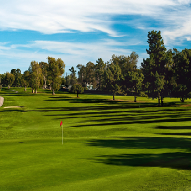
I performed the landscape classification for a single 2020 NAIP tile. This is about a 6 km x 6 km area within the greater Long Beach Water service area. The workflow can eventually be scaled to analyze an water supplier's entire service area. The location and detail of the NAIP tile is shown below.
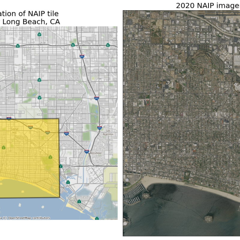
Notice above that there are several properties with large landscaped areas. Golf courses, a park, and sports fields are identifiable from this view. These are the landscaped areas we are interested in identifying.
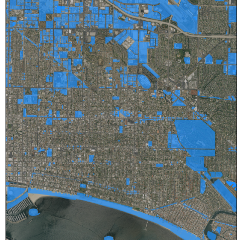
Overlaying commercial parcel boundaries
Long Beach falls within Los Angeles County. The County maintains a shapefile of all parcels within its boundaries. This file also contains information about the property, including whether it is a CII or residential property. We can overlay a shapefile of CII property boundaries onto our test tile image, and eventually use these polygons to calculate the total CII landscaped area.
Classifying imagery to identify vegetation
For the land cover classification, I used the RandomForest (Brieman 2001) ensemble decision tree algorithm by Leo Breiman and Adele Cutler, outlined in the random-forest-classification tutorial. Random Forest utilizes the scikit-learn Python library.
This is a supervised classification approach, which means training data are input to the model so it can classify other pixels in the image as "vegetation," "water," or "other."
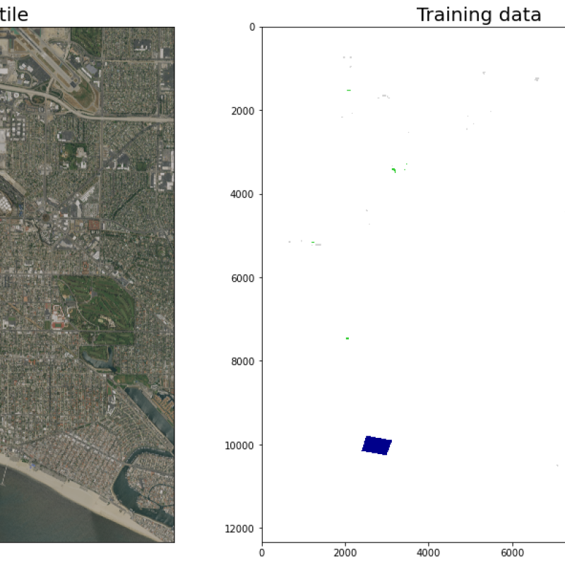
Examining training data
Below is a sample of the training polygons used to supervise the model. These polygons are drawn on areas that are clearly turf grass, trees, or shrubs, and will tell the model what to "look for" in the other image pixels.
Preparing NAIP bands and NDVI
Now that the model knows where in space these vegetation pixels are, it can identify unique properties of these pixels, using:
- the color image itself, which is composed of red, green, and blue bands
- a fourth band, near infrared, which is collected along with the RGB bands
- a layer that contains the Normalized Difference Vegetation Index (NDVI) for each pixel
- a layer that contains the Normalized Difference Water Index (NDWI) value for each pixel
The below plot shows each of these feature layers which are input into the classification model.
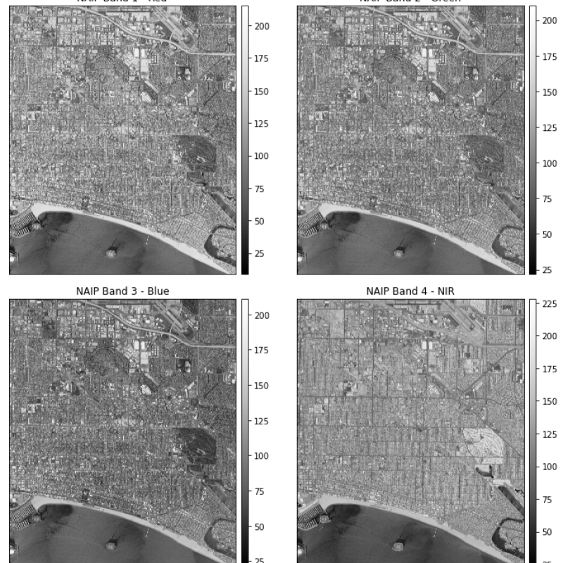
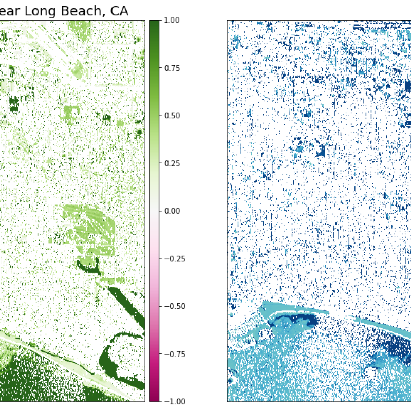
The combination of the above data will help the model identify the unique "signature" of the vegetation pixels.
Preparing the classifier by exploring training data
Each pixel in the training data corresponds to a pixel in each of the feature layers above. We can explore
The number of training pixels in each class are shown below.
| class | number of training pixels | |
|---|---|---|
| 0 | 1 | 69343 |
| 1 | 2 | 256882 |
| 2 | 3 | 46547 |
If we plot the spectral signature (from the 4 NAIP bands) of each pixel, grouped by class, we can see that vegetation pixels have a clear signature, but water and "other" pixels are indistinguishable.
This is where the NDVI and NDWI feature layers provide more helpful information for the model to distinguish between the two classes.

Train model on all training data
We have now seen the two inputs to the RandomForestClassifier model:
- the training data
- a stack of the feature arrays (NAIP bands, NDVI, and NDWI)
We can now train the model on all data.
Cross-validation
In order to assess the accuracy of the model we created above, we perform a "cross-validation." This involves excluding some of the training data from the model fit, then using that new model to check its performance on the remaining excluded training data.
Run classifier on NAIP tile
Now that the model has been trained, we can use it to classify all of the pixels in the NAIP tile.
Below is the resulting final classified image!
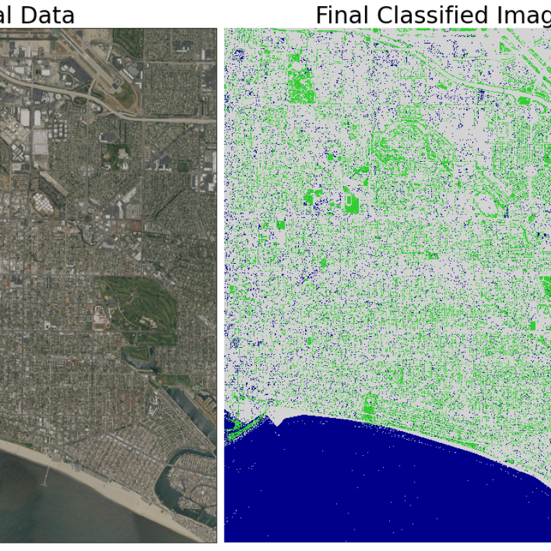
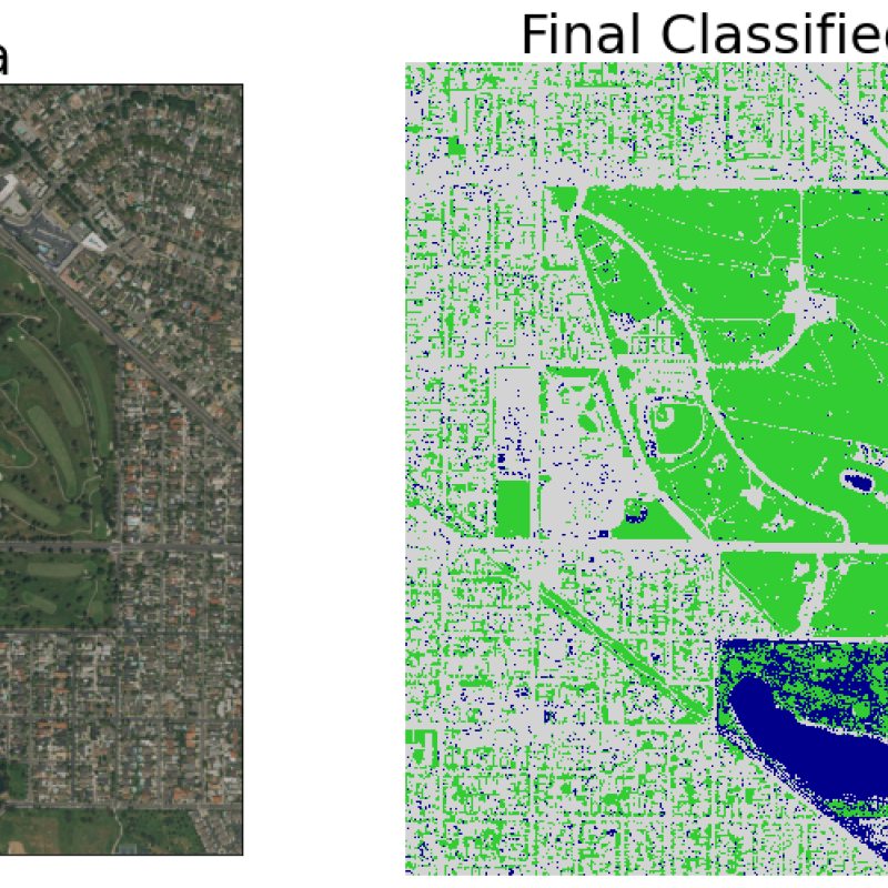
We can zoom in and see the classified image in more detail - below is an area with a golf course, sports fields, a pond, and some residential areas.
The model did a pretty good job picking out the vegetation pixels from the rest. It seemed to struggle to differentiate between water and "other" pixels, but since we are only interested in the vegetation pixels, these results are sufficient.
So which features were the most important in helping the model classify the image?
Below the "feature importance scores" are shown. The feature numbers are as follows:
- Feature 1 - red band
- Feature 2 - green band
- Feature 3 - blue band
- Feature 4 - NIR band
- Feature 5 - NDVI
- Feature 6 - NDWI
The features with the highest importance scores were NDVI and NIR.
Conclusions
Instead of manually measuring every CII property in their service areas, water suppliers can use this method to estimate their total CII landscaped area. They can then use this calculated area to create and maintain water budgets in accordance with California legislation.
To perform this classification across an entire service area, the user will need to make some adjustments to the workflow including:
- pulling all NAIP tiles that will cover the extent of their service area
- clipping these tiles to the boundaries of their service area
- performing the classification and calculation steps for each clipped tile
- summing the total landscaped area across all tiles