Jerry Gammie, and Cibele Amaral
Nayani Ilangakoon, Anna LoPresti, Laura Dee, Claire Monteleoni, Natasha Stavros

The terrible effects of wildfires are becoming increasingly inescapable, whether we are actually directly affected by them or read about their devastation in the news, breathe their smoke, or are impacted in another indirect way. This problem will be exacerbated by climate change. However, ecological research suggests that prescribed burns can help. Of course, prescribed burns are still fires and have their own effects - the goal of this project is to predict some of them. We want to use machine learning to predict proxies for ecological functions after a burn.
    This project builds on previous work I have done with Earth Lab, in which I developed a pipeline for harmonizing multi-scale remote sensing data into data cubes with 5 meter sampling, then using them to predict ECOSTRESS Water Use Efficiency with machine learning. Harmonizing the data ended up being the hard problem - I wanted to use very powerful model architectures designed for image data, which on the surface was a similar 2 dimensional format to the remote sensing data. However, our data included raster data at different resolutions and even point data. We ultimately built our data cubes with 5m sampling because that was the greatest common divisor of all the resolutions involved. 
    With the move to predicting outcomes of wildfires came an expansion of the scope of the project. Instead of predicting WUE over a region of the front range, we would predict above ground biomass, ECOSTRESS ESI, and WUE first across the state of Colorado and then across the western United States. We would make these predictions from elevation, slope, aspect, and land cover (all at 30m resolution), alongside new data like forest stand age (at 1km resolution). We realized that the previous 5m subsampling method would make data storage difficult or even infeasible with more samples because of the huge dimensionality of the data - around 17,000 input parameters in every sample! 

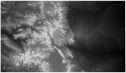
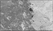
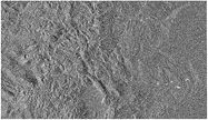
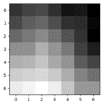
Above, from top: Elevation, land cover, and aspect over the state of Colorado

    We experimented with reducing the resolution of the sampling to 30 meters, creating 4 by 4 by 66 data cubes, a 16-times reduction in the dimensionality. We found that this greatly sped training of models. In theory, there is a tradeoff between model quality and training time with the number of features. One expects a model that uses fewer features will train faster but will ultimately  perform worse. However, in our 5 meter sampling strategy, we were only capturing a small amount of extra information while greatly increasing the number of features. I believe that this ended up bogging down the model and made it difficult for the model to feasibly reach a level of performance on par with what it could do with fewer parameters. 
    Coarser sampling ended up being a win-win, but I felt that the strategy may still be creating sub-optimum data cubes because of mismatches in the resolution and alignment of the data that we were sampling. This motivated the next part of the project: an interpolation step to align the data and resolve scale differences. I experimented with coarse sampling and a basic linear interpolation method to create the data cubes and found that the predictive model performed slightly better on the interpolated data, but both methods led to better performance than the original 5m sampling strategy.

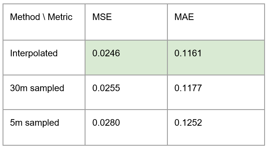
Above, I trained a random forest on datasets generated with each of the three methods and computed their mean squared error and their mean absolute error. Lower is better for both metrics. The interpolated data allowed for the best model performance. This was great too - we got better performance with the same data size - but I naturally wanted to try applying machine learning to the interpolation to see if we could do even better. 
    I set up the interpolation as an upscaling problem, where the models were to increase the resolution of the image before sampling or basic interpolation was carried out on the higher resolution predicted samples. I took a 30m dataset and averaged over 3 by 3 squares to create paired low resolution and high resolution data. I used this to train the models and got poor results - the predicted high resolution images often contained artifacts and did not look very close to the actual data. I think with more training, more data, and different and better model architectures could have improved performance a lot here, but I rethought this strategy before I learned more about upscaling and improved the models.

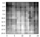
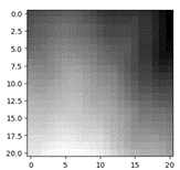
Above, from top: The low resolution (7x7) sample, the upscaled sample, and the original high resolution (21x21) sample

    Even so, when I trained classifiers on data cubes produced with the supervised method, they performed better than the same classifier trained on data cubes made with sampling or linear interpolation. The upscaling models may not have produced very convincing high resolution data but it appeared that they were still capturing and including some extra information that was benefiting the classifier. Ultimately, though, this confusing result led me to rethink my whole approach.
    We currently had a two-step approach where we first generated data cubes and then made predictions from them. On both ends, I was using convolutional neural nets, with different and disconnected goals. With this approach, gradient descent and weight updates that improved the ultimate predictions stopped at the interpolated data. There was no way to improve the weights in the upscaling step based on the predictions even though the ultimate goal of upscaling was to make better predictions.

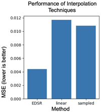
Above: comparison of the performance of a random forest model trained on data generated with each interpolation method. Note that this comparison is on a small subset of the data (over samples and features), leading to inflated performance.

I dealt with this by adopting a one-step approach. In a departure from my previous work, the model would take un-harmonized data as inputs and directly use it to make predictions. Harmonization, instead of being explicitly required, would have to take place implicitly within the model. This left our data cubes as “data pyramids” instead, where over a 1km sample the coarsest (1km resolution) data would have only 1 entry while the finest (30m resolution) data would have 34. I also realized at this point that we would be using the same data pyramids to predict three response variables - so why not adopt a multitask approach and predict them at the same time. In theory, this strategy leads to more robust and better trained neural nets. It also meant that we would make predictions on the 1km resolution above ground biomass data and all the 70m ECOSTRESS pixels within that square kilometer at the same time. 
    At this point, the model is taking shape: it takes each input layer at its original resolution, combines them within the model, and then expands back out to make two-dimensional predictions on all three response variables at the same time. The final idea came, in part, from models like U-net, where over subsequent convolutional layers it extracts more and more general features from the data. Our data is already composed of more and less general features, based on their resolution. So the model combines the data at different stages of the convolutional layers, with finer data being combined first and coarser data being combined last. The final model architecture is illustrated below.

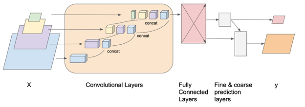
Above: Model architecture. Coarser raster data is represented by smaller squares on the top.

    I have not yet adequately tested this model or developed baselines to compare it to. The main properties of this model are multitasking, combining the data layers in a cascading manner within the convolutional layers, and data pyramids instead of data cubes. I aim to develop baselines for all of these properties to compare their performance to that of our model. For multitasking baselines, I remove the prediction layers for all but one response variable and train a separate model for each response variable. I compare some preliminary performance results below. The multitask model achieves similar or better performance across the board.

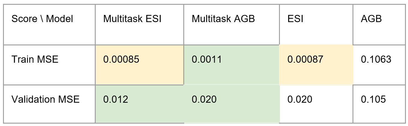
Above: Comparison of predictions from multitask model and single task models. The multitask model achieves similar or better validation MSE over both response variables.

    There is an additional caveat to this work: the data that I have been working so far, and that I got the above results with, is over the entire state of Colorado. The ultimate plan for this work is to train only on wildfire burn areas, which will greatly reduce the sample size. I don’t know how this will effect model performance and whether our model will be right for the job. I would expect a wider performance margin between our model and similar single task models because multitasking is increasing the amount of feedback that the model gets. Beyond that, I am not sure.
Still, I have expanded and improved my machine learning pipeline for remote sensing data, from basic pre-processing to building data cubes, interpolation, and more. This will be made publicly available. And, of course, I have developed a novel model that is already performing well and is ready to be tested against a variety of baselines. Thank you to Earth Lab for the great summer!