Intro

Thermal imaging cameras mounted on drones can detect hot spots on electrical systems prior to equipment failure. These failures result in financial costs to the utility companies, inconvenience to customers, and safety issues to the electrical linemen.

Thermal images are often acquired while the operator is focused on taking standard RGB images, resulting in thermal images that are blacked-out, saturated, or blurred. All thermal images are sent to a thermographer, who charges the customer to identify these bad images in addition to analyzing the good ones.

Objective

I decided to try different machine learning techniques to classify the data for several reasons. For one, using Sklearn allowed me to apply some of the same code across different models. Additionally, adjusting the parameters and/or applying the models to additional training data can improve the results. Lastly, it saves costs by automating the process of image classification. Let's see how we can train one or more machine learning or predictive models to identify the bad images, while minimizing false negatives (ie. misidentifying the good images). The best model will be determined by its confusion matrix.

import rasterio as rio
import numpy as np
import pandas as pd
import os
from glob import glob
import matplotlib.pyplot as plt
%matplotlib inline
import cv2

from sklearn.model_selection import train_test_split
from sklearn.ensemble import RandomForestClassifier, GradientBoostingClassifier
from sklearn import linear_model
from sklearn import svm
from sklearn.metrics import classification_report
from sklearn.metrics import accuracy_score
from sklearn.metrics import confusion_matrix

import sys
sys.path.insert(0, 'C:/Users/micha/github/uav-image-analysis/scripts/')
import fit_models

os.chdir("/Users/micha/ea-applications")

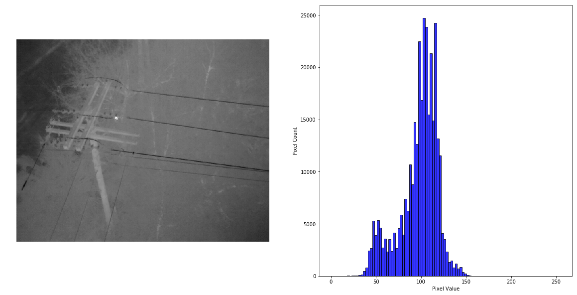
Good Image

Here is a typical thermal image of powerlines, utility pole, and equipment. Note the hot-spot on one of the connections.

path = glob("data/training-test-images/Thermal/2019-02-16/101MEDIA/DJI_0480.jpg")

for im in path:
    with rio.open(im) as src:
        image = src.read()

        fig,ax = plt.subplots(1,2,figsize=(20,10))
        ax[0].axis('off')
        ax[0].imshow(image[0], cmap = "gray")
        ax[1].hist(image[0].flatten(), bins=100, facecolor='b', edgecolor='k', alpha=.8)
        ax[1].set(xlabel="Pixel Value", ylabel="Pixel Count")
        plt.show()

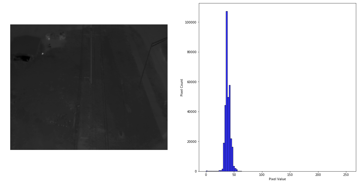
Blacked-Out Image

Note the histogram skewed to the left with highly concentrated brightness values for this blacked-out image.

path = glob("data/training-test-images/Thermal/2019-02-16/101MEDIA/DJI_0116.jpg")

for im in path:
    with rio.open(im) as src:
        image = src.read()

        fig,ax = plt.subplots(1,2,figsize=(20,10))
        ax[0].axis('off')
        ax[0].imshow(image[0], cmap = "gray")
        ax[1].hist(image[0].flatten(), bins=100, facecolor='b', edgecolor='k', alpha=.8)
        ax[1].set(xlabel="Pixel Value", ylabel="Pixel Count")
        plt.show()

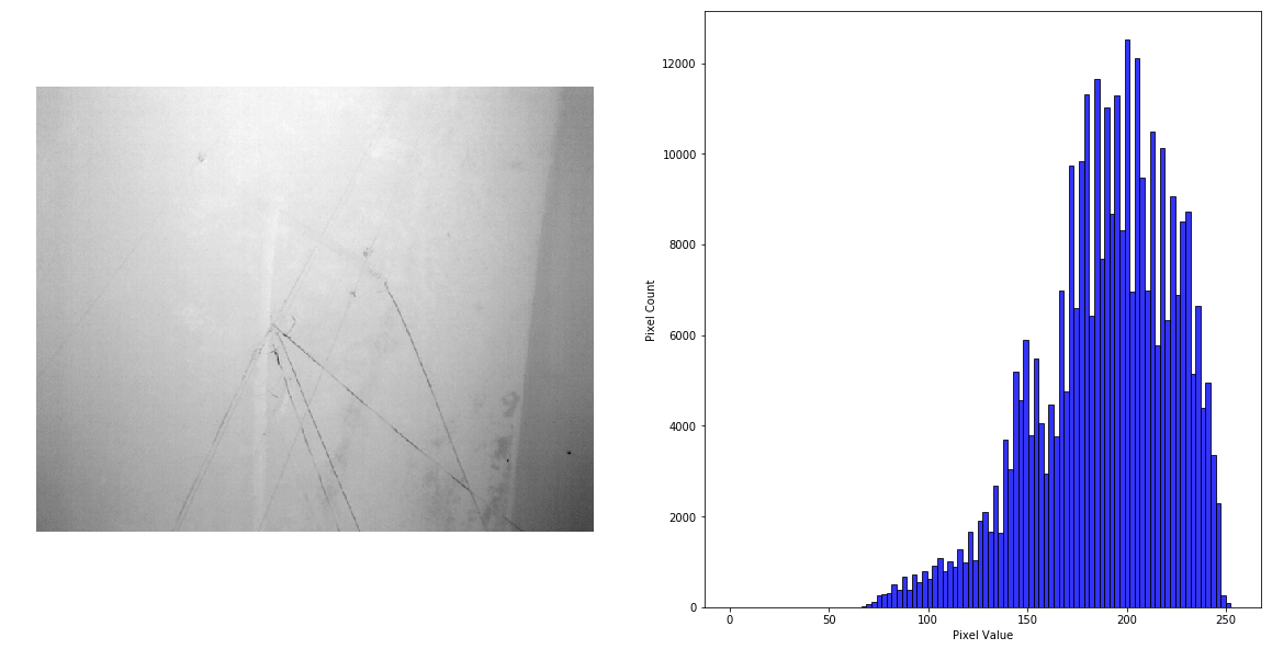
Saturated Image

Brightness values for saturated images tend to skew to the right side of the histogram.

path = glob("data/training-test-images/Thermal/2019-02-17/100MEDIA/DJI_0001.jpg")

for im in path:
    with rio.open(im) as src:
        image = src.read()

        fig,ax = plt.subplots(1,2,figsize=(20,10))
        ax[0].axis('off')
        ax[0].imshow(image[0], cmap = "gray")
        ax[1].hist(image[0].flatten(), bins=100, facecolor='b', edgecolor='k', alpha=.8)
        ax[1].set(xlabel="Pixel Value", ylabel="Pixel Count")
        plt.show()

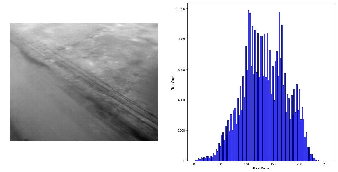
Blurred Image

A blurred image, however, does not always differentiate well from an acceptable image.

path = glob("data/training-test-images/Thermal/2019-02-16/101MEDIA/DJI_0102.jpg")

for im in path:
    with rio.open(im) as src:
        image = src.read()

        fig,ax = plt.subplots(1,2,figsize=(20,10))
        ax[0].axis('off')
        ax[0].imshow(image[0], cmap = "gray")
        ax[1].hist(image[0].flatten(), bins=100, facecolor='b', edgecolor='k', alpha=.8)
        ax[1].set(xlabel="Pixel Value", ylabel="Pixel Count")
        plt.show()

Challenges

The data provided to me was unbalanced, with good images highly outnumbering all of the bad ones combined. However, other datasets may contain more bad images. The lack of data was an impediment to applying the Convolutional Neural Net (CNN) model in addition to the others. And while classification of "Good" and "Blacked-Out" images showed a high level of accuracy, the learning models did not perform as well for the "Saturated" and "Blurry" images.

Application

I applied different machine learning and predictive models to the data to see which one is best for classifying the images, including Support Vector Machine (SVM), Logistic Regression, Random Forest, and Gradient Boosting (for more information on the different methods, see my GitHub page https://github.com/mlevis1/uav-image-analysis).

# Create dataframe from test-images.csv image names and labels
df_train = pd.read_csv('/Users/micha/ea-applications/data/test-images.csv')
# Set path to training/test image folders
paths = '/Users/micha/ea-applications/data/training-test-images/Thermal/mytest/*MEDIA/'
# Read data from image files
train_images,_ = fit_models.read_images(paths)
y = np.array(df_train['Label'])
y = df_train['Label'].values
# Split data into 60% training images and 40% testing images
X_train, X_test, y_train, y_test = train_test_split(train_images, y, random_state=42, test_size=0.4)

(431, 327680)

# Run random forest classifier
model = RandomForestClassifier()
# Train model and get model predictions and probabilities
model_logistic, probabilities, y_pred = fit_models.supervised_models(model, X_train, y_train, X_test, y_test)

Results

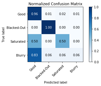
The Random Forest Classifier is similar to a decision tree analysis, and provided the best accuracy with the test data as shown below. Recall is the best measure of accuracy when avoiding false negatives is a key objective.

Confusion Matrix

The confusion matrix shows the performance of the learning model, in this case the Random Forest Classifier. You can see the high level of accuracy for "Good" and "Blacked-Out" images, while only half of "Saturated" images tested accurately, and almost all of the "Blurry" images were misclassified as "Good".

class_labels=['Good', 'Blacked-Out', 'Saturated', 'Blurry']

np.set_printoptions(precision=2)

# Plot normalized confusion matrix
fit_models.plot_confusion_matrix(y_test, y_pred, classes=class_labels, normalize=True,
                      title='Normalized Confusion Matrix')

plt.show()

Conclusion

I'll save the trained Random Forest Classifier for future application to new, unlabeled images. Given the poor performance of the "Saturated" and "Blurry" categories, I considered removing them from the model. However, they are accurate some of the time (50% for "Saturated"), without significant effect on the outcome for "Good" images. Additional testing with new data would allow additional validation by an actual person. I would also like obtain additional training data in order to further expore the Convolutional Neural Net (CNN) learning model.