Development in the Hinderlands
By Caitlin Mc Shane & Michelle Roby
Project Introduction
As urban development occurs, areas that were once natural environments are replaced with manmade infrastructure. This requires the removal of vegetation. With rapid urbanization, more and more natural environments are being converted into city structures. Monitoring changes in vegetation could be a helpful indicator to show how cities are developing. This monitoring could lead to a better understanding of urban development that can then help policy makers and city planners improve future urban planning. With population growth and more people moving to cities, proper urban planning is vital for creating enjoyable living environments.
There has been some past research on how NDVI and plant productivity changes with urbanization overtime (Esau et al., 2016 & Beck & Goetz, 2011). In our study, we wanted to explore if NDVI could be used as an early signal to urban development. We hoped that the results of our analysis could indicate changes that the natural environment undergoes during the development process. Our specific research question is as follows:
Is there a correlation between changes in Normalized Difference Vegetation Index (NDVI)* and structural intensity for an urban environment?
We predict that a greater change in structural intensity will correlate with a greater decrease in greenness (measured by the NDVI value).
*NOTE: NDVI is a common remote sensing technique used to determine the health or density of vegetation across an area.
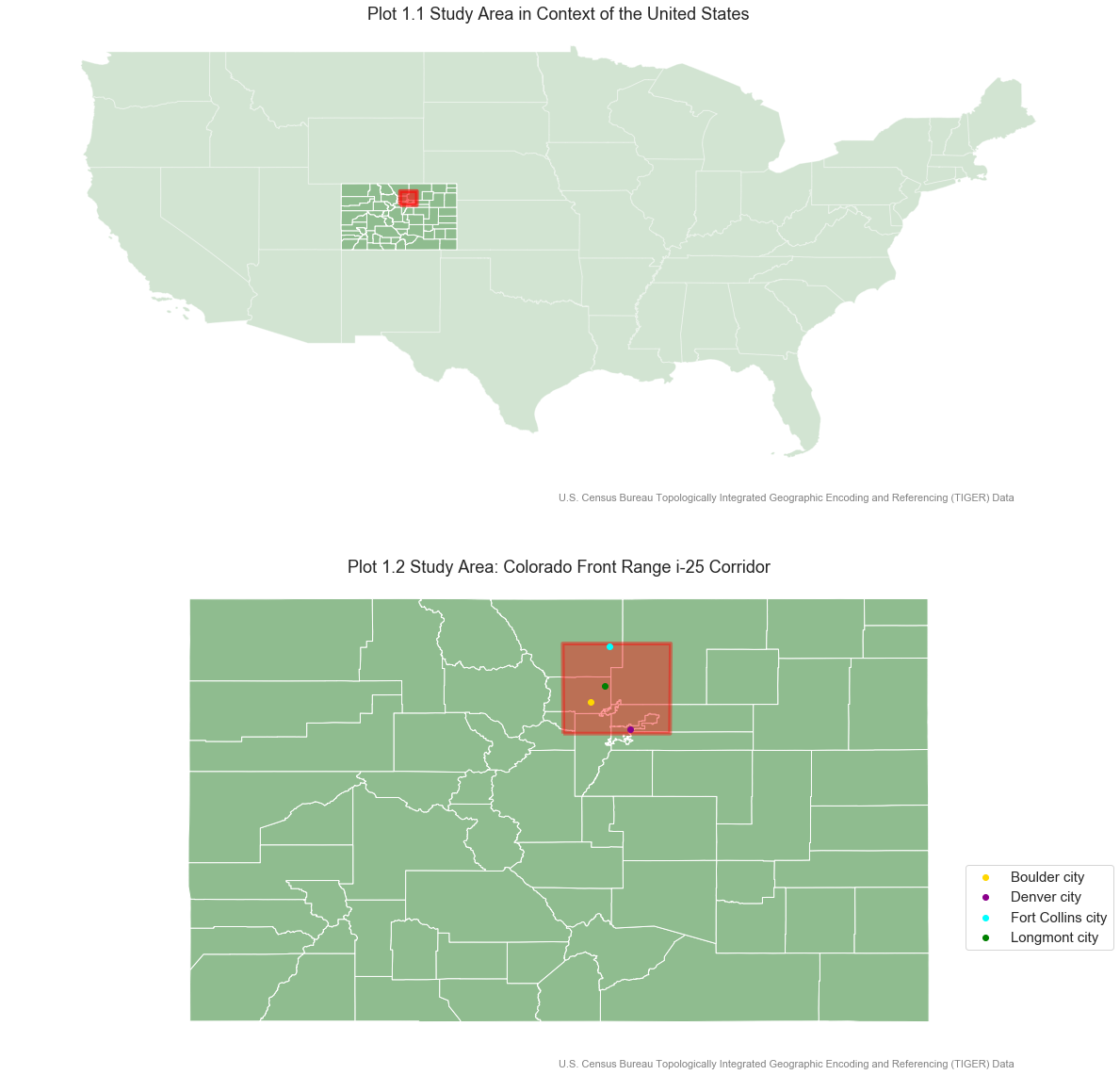
Plot 1: The Study Area
The study area for this analysis is the I25 corridor in the northern Colorado Front Range (red box). This area was selected because of its influx of development in the past few decades.
About the Data
There are two data sources for this analysis. The main data used is the Landsat 5 raster files. The bands used are 3 (red) and 4 (near infrared) to calculate Normalized Difference Vegetation Indices (NDVI). The second data source that is used are from the HISDAC-US dataset. The HISDAC-US data has a temporal scale of 5 years based off annually collected Zillow data that was aggregated into 5 year time slices. During the processing, all of the data is clipped down to the size of the study area.
Landsat 5 Data Processing
To determine the levels and distribution of the vegetation for each year, an NDVI (Normalized Difference Vegetation Index) was calculated for each year. Then, the difference in NDVI between years was calculated. The final outputs from this processing are four NDVI difference images showing the change in vegetation greenness for each of our time slices.
Hisdac-US Data Processing
The HISDAC-US data was projected to the same Coordinate Reference System as the Landsat 5 NDVI data. Then, the NDVI data (smaller, 30x30 meter pixels) was reshaped to match the shape of the HISDAC-US arrays (larger, 250x250 meter pixels) for comparison.
We decided to focus on areas that had no built environment at the start of our study in 1985. For the rest of our analysis, we did analysis on only these initial ‘no built’ areas.
In the 'no built environment' pixels, the following were calculated for each time slice:
- the percent change in structural intensity
- NDVI difference values for each pixel
Data Exploration and Visualization
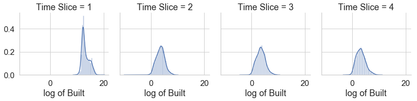
Plot 2: Data Distribution
The density distributions for the built change have a sharp peak and skew towards the right. To normalize the structural intensity change, the log of the 'Built Change' variable was calculated. Time slice 1 (change from 1985 to 1990) has an interesting distribution that appears to have a sample statistically different from the subsequent time slices.
NOTE: Time Slice 2 = 1990-1995 Time Slice 3 = 1995-2000 Time Slice 4 = 2000-2005
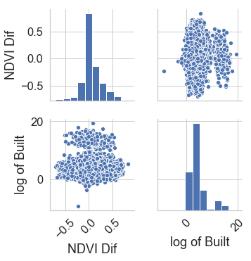
Plot 3: Pair Plot
In order to have a general understanding on how the data behaves, we take a look at our primary variables in a pair plot that allows us to visualize the data in terms of distribution and relationships. To normalize our data, we took the log of the 'Built Change' variable. The bimodal distribution of the 'log of Built' feature is reflected in the scatter plot depicting the relationship between 'NDVI Dif' and 'log of Built'. The clustering of NDVI difference values around the peak of the 'log of Built' bimodal distribution requires further investigation.
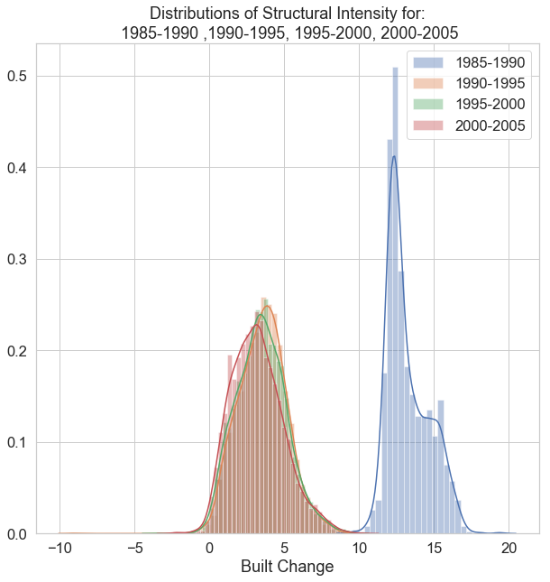
Plot 4: Built Change for Each Time Slice
To see if the different time slices are comparable, we compared the distributions of each time slice to each other. Time slice 1, the slice reflecting change in 1985-1990 (blue), shows a significant difference in domain compared to the other years. This makes it difficult to directly compare time slices. Instead of further manipulating the data, we decided to look at the relationship between NDVI differences and changes to the built environment for each time slice.
Plot 5: Regression Models
The regression models for each time slice looking at the response of NDVI to the changes in the built environment are plotted below. A trend line was added to visualize any distinct relationships between the variables. There are some interesting observations that result from these plots.
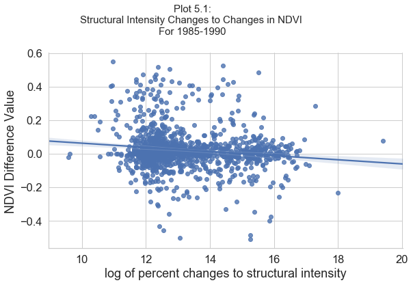
Plot 5.1: 1985 to 1990
Shows a distinct negative relationship between structural changes and NDVI difference values. There also appears to be several clusters of NDVI values along the range of structural intensity.
A cluster of NDVI exists in the logb(12) - logb(13) range. Another, less dense cluster of NDVI values exists in the logb(15) to logb(17) range. The third cluster shows a positive relationship between NDVI and 'log of Built' in the -0.6 - 0 for NDVI and logb(15)-logb(17) range.
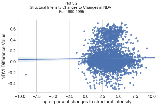
Plot 5.2: 1990 to 1995
The mean for changes to the built environment shifts downward and values for built changes cluster between approx logb(0)-logb(10). The NDVI values respond with tighter clustering and lower range of values.There appears to be two dominant clusters with NDVI in the range -0.2 - 0.2 and 0.4-0.6.
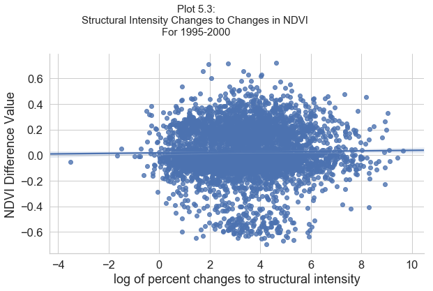
Plot 5.3: 1995 to 2000
Two clusters of NDVI values appear that have overlapping built change ranges. The top cluster of NDVI values displays more range than the bottom cluster of values. It appears that these clusters exist in all graphs but the fourth and swap places each time slice.
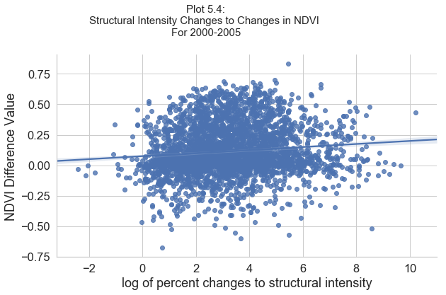
Plot 5.4: 2000 to 2005
The values start to form a denser cluster that starts trending positively, which is in contrast to the first signal in 1985-1990. This is interesting as that is the inverse relationship to what we would expect.
Correlation Tests
After running each time slice through a regression test, the only slice with statistically significant results was the fourth time slice (2000-2005). For this time slice, the results of the R squared and p-value indicate the relationship between NDVI and changes to the built environment explains roughly 20% of the variance in the data. Although the other time slices has significant p-values, they had R squared values for these times were very low, meaning that the change in NDVI is not strongly correlated with changes in the structural intensity.
| Dep. Variable: | NDVI Dif | R-squared: | 0.231 |
|---|---|---|---|
| Model: | OLS | Adj. R-squared: | 0.231 |
| Method: | Least Squares | F-statistic: | 1072. |
| Date: | Sun, 16 Dec 2018 | Prob (F-statistic): | 8.75e-206 |
| Time: | 21:26:42 | Log-Likelihood: | 619.52 |
| No. Observations: | 3573 | AIC: | -1237. |
| Df Residuals: | 3572 | BIC: | -1231. |
| Df Model: | 1 | ||
| Covariance Type: | nonrobust |
| coef | std err | t | P>|t| | [0.025 | 0.975] | |
|---|---|---|---|---|---|---|
| log of Built | 0.0306 | 0.001 | 32.735 | 0.000 | 0.029 | 0.032 |
| Omnibus: | 57.327 | Durbin-Watson: | 1.063 |
|---|---|---|---|
| Prob(Omnibus): | 0.000 | Jarque-Bera (JB): | 61.722 |
| Skew: | 0.285 | Prob(JB): | 3.96e-14 |
| Kurtosis: | 3.301 | Cond. No. | 1.00 |
Warnings:
[1] Standard Errors assume that the covariance matrix of the errors is correctly specified.
Summary and Conclusions
The results of this study were surprising. We had expected to find significant decreases to NDVI values where development was occurring, however we discovered that the pixels that had the highest changes to structural intensity were associated with the smallest changes in NDVI. We found that every pixel with significant changes to the built environment contained very small changes to NDVI that were only statistically significant at the initial change.
We conclude that there is potentially a signal in changes to NDVI prior to urbanization for areas that had little to no built environment. However, the nature of these changes and their relationship to structural intensity needs to be researched further. Other interesting findings were clusters of positive change to NDVI with increasing structural intensity, which may be attributed to human planting as the urban environment develops. There are clear clusters of values indicating other relationships and variables at play. The results of the study also show possible efficacy in using the relationship between NDVI change and structural intensity to delineate the boundaries of urban clusters as the majority of development appears to be at the edges of a cluster.