In almost every field (and especially in any kind of data science), there will be times when we wish to estimate data we don’t have by using the data that we do have. Given the plethora of machine learning algorithms and the similarly-daunting number of implementations of these algorithms (in different languages, packages, etc), it can be difficult to know where to start. This post shares my biggest takeaways from diving into using some of these tools, in the context of estimating air pollution from wildfires over the western US.

Science Motives

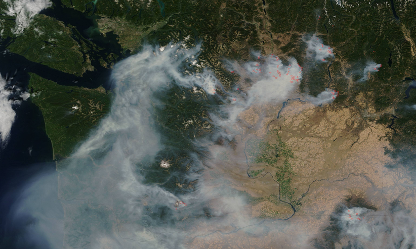
Since September 2017 I’ve worked on the Environmental Health Team in Earth Lab, investigating the impacts of exposure to air pollution from wildfires on human respiratory and cardiovascular health in the western US. To study the health impacts of air pollution, we have to know how much air pollution there was at each time and location of interest. (For the health analysis, we can then determine statistical relationships between quantities of air pollution and medical records.) However, a relatively sparse network of regulatory-standard air quality monitors does not offer continuous measurements of air quality across the western US. 

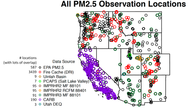
To estimate air pollution (specifically PM2.5, fine particulate matter -- which is an air pollutant of primary concern for health) across the western US from 2008-2018, my team is employing a collection of of machine learning and spatial modeling techniques (described in the following sections). Read here about the variety of environmental data sets (meteorological variables, satellite imagery, etc) that my team is using, as well as the policy implications of this research.

Machine Learning with R caret and caretEnsemble packages

In my previous blog post, Wildfire Air Pollution and Health, I introduced the machine learning techniques I was just starting to use for this project, as well as some general machine learning concepts and terminology, such as cross-validation and tuning parameters. Here, I’ll share some of my experiences from applying these techniques (and others) to our data. My team and I are still finishing processing some environmental variables in our 2008-2018 coverage of the western US. However, I have been experimenting with a subset of the data which covers the 11 western states from early 2008 through the end of 2010, and includes MODIS MAIAC and GASP (satellite sensors) Aerosol Optical Depth (AOD), wind speed vectors, atmospheric pressure, temperature and humidity, elevation, and proximity to major roadways. 

I have been working in the programming language R, primarily using the caret and caretEnsemble packages to perform machine learning. Initially, I became familiar with caret through the “Machine Learning Toolbox” [in R] module on DataCamp. I also learned lots from Zev Ross’s “Predictive modeling and machine learning in R with the caret package” tutorial. 

Caret allows me to easily perform the following tasks (with functions underlined):

• sample separate training and testing data (in experimentation thus far, I have used a 90:10 ratio of training to testing data)
• build a grid of tuning parameters (iterating through these parameters allows for optimization of the model during training) 
• resample folds of my training data, which are then used in cross validation (this helps avoid overfitting the model on the training data) 
• build a trainControl object which specifies all the cross validation arguments, including the number of times I want to repeat model fitting
• train the model, specifying the model structure, performance metric (Root Mean Squared Error, Accuracy, etc), preferred machine learning algorithm, and any other parameters relevant for that algorithm. For instance, Ranger (a highly efficient random forest algorithm) accepts arguments for the number of decision trees and the importance rule, which determines how variable importance is calculated.
• List variable importance (via the varImp function)
• predict at new locations, given new predictor data at the new locations

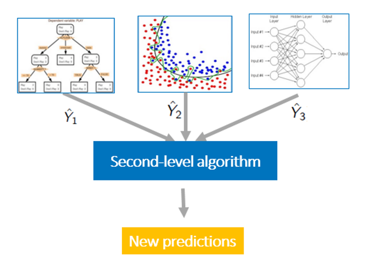
The steps above harness one kind of machine learning algorithm at a time. An extension of single-algorithm machine learning is to create a pooled model called an ensemble or stack. In essence, we run a bunch of individual models with different algorithms, and then run another algorithm (which I refer to as the “stacker algorithm”) on the output from the individual models. By blending the results from several machine learning algorithms together, an ensemble is able to capture more variation in the data than any single algorithm could, leading to higher prediction accuracy. 

The caretEnsemble package is especially user-friendly because it provides ensemble methods which are compatible with normal caret methods, such as using a trainControl object. The caretEnsemble package allows me to do the following (with functions, again, underlined):

• Run a set of machine learning algorithms (typically two to four algorithms) on the data, and store the resulting set of models in a caretList object
• Blend models using a generalized linear model (glm) as the stacker algorithm using caretEnsemble
• Blend models using any caret algorithm (glm, gbm, random forest, etc) as the stacker algorithm using caretStack

Here is a more detailed Introduction to caretEnsemble. I also recommend this code example for how to build a stack using caretEnsemble. This tutorial is for classification (predicting discrete classes), but adapting it for regression (predicting numerical values from a continuous distribution) is quite straightforward.

Fumbling with Ensembles (Some Takeaways from My Experience)

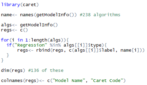
In machine learning, classification refers to sorting data into discrete classes, whereas regression refers to estimating values from a continuous distribution. My project necessitates using regression to estimate the exact concentration of PM2.5. Thus, to start my machine learning odyssey, I examined the whole list of caret algorithms that support regression (as opposed to classification only). There are 136 in total, which I found using the following code:

Eventually, I selected eleven algorithms, refining the list by trying to get at least one from each well-known category of machine learning regression algorithms, and researching which algorithms within each category performed the best. Here is the list of algorithms I used, along with the name of each algorithm as it is called in the caret package:

• Generalized Linear Model = “glm” 
• Generalized Additive Model using Splines = “bam”
• Stochastic Gradient Boosting = “gbm”
• Random Forest = “ranger”
• Supervised Principal Component Analysis = “superpc”
• Multi-Layer Perceptron, with multiple layers = “mlpML”
• Gaussian Process with Radial Basis Function Kernel = “gaussprRadial”
• Support Vector Machines with Radial Basis Function Kernel = “svmRadial”
• eXtreme Gradient Boosting = “xgbTree”
• GLM with Elastic Net Regression = “glmnet”
• Bagged MARS (Multivariate Adaptive Regression Splines) = “bagEarth”

Observations from my experimentation with these algorithms on my team’s air quality and environmental predictors data include:

• Regarding individual algorithms:
  • Ranger always performs the best, followed by gbm-gaussprRadial-xgbTree (these three are very close), and svmRadial 
  • Then bagEarth
  • Then glmnet and glm -- these perform about the same (not well), but they are quick so it wouldn’t hurt much to include them in an ensemble
• Regarding stacker algorithms:
  • Glm performs worst (basically achieves the R2 of the best individual algorithm)
  • Ranger performs best (increases the R2 several percentages above the best individual algorithm), but takes a long time
    • Reducing the number of repetitions (which often results in the same choice of tuning parameters) makes this a more viable option
  • Gbm performs nearly as well as Ranger in the role of the stacker, and takes less time (even with 3 repetitions)
• Regarding tuning:
  • Increasing the number of resamples (more than 10) in the trainControl object helps a bit, but takes a lot longer 
  • The tuneLength parameter doesn’t seem to change the results that much (there are only slight improvements in R2 and RMSE)

Because I observed that a solo Ranger model always performed nearly as well (and ran much faster) compared to a stack of three or four algorithms, I decided to just use Ranger in subsequent testing. Other modelers with different data sets and computational restrictions may well choose a different strategy.  

Report Cards: How Each Machine Learning Model Performed 

To evaluate each model, I look at both the Root Mean Squared Error (RMSE) in predicted versus actual PM2.5 concentrations and the R2 value (which represents the percentage of variation in the training data that the model is explaining) on both the training and testing data sets. When modeling, we strive for lower RMSE and higher R2, both of which mean that our results are more accurate. Not surprisingly, the training RMSE and R2 values were lower and higher respectively (better) than their testing counterparts, which shows that the kind of cross-validation we can easily implement with caret is still not as honest as holding out an entirely separate testing set (as I did at the beginning using the sample function). Read more here about the practice of using separate training and testing data.

Another way scientists often evaluate such models is by calculating “spatiotemporal R2 ”. This metric describes the model performance when we hold out entire geographic regions or time periods from the training data, and then test on these held-out regions. The argument is that this procedure more realistically evaluates the model’s performance when predicting at locations for which we have no past or present monitoring data. I implemented this procedure using caret’s groupKFold function. Unsurprisingly, the spatiotemporal R2 values are usually lower (worse) than their regular R2 counterparts. 

Another key way of evaluating model performance, especially when dealing with spatial and/or temporal data, is to visualize the output of the model using a relevant plot. I have not included specific numerical results or plots here due to the in-progress status of this modeling project. 

Slice and Dice: Spatiotemporal Subsetting

Although fitting one huge (“global”) model to the 11 western states from 2008-2018 could be useful, from early on it became clear that smaller (“local”) models focusing on different geographic regions and time periods would yield much higher accuracy. Thus far, I’ve experimented with models on geographic quarters of our study region, the four seasons, and combinations of these spatial and temporal subsets. Due to a high density of both air pollution and air quality monitors, summers in the southwestern quarter of our study region (which ends up being California plus some fractions of the surrounding states) make for the best modeling results. Other regions and seasons prove more challenging due to greater variability and lack of data. However, typically the more data we have, the better the algorithm can learn significant patterns, so training on more data (once we’ve finished processing everything) will likely improve the results in other spatiotemporal subsets. 

Kriging on the Residuals

Another way that I attempted to improve our air pollution predictions and understanding of spatiotemporal trends in the data was to use kriging on the residuals (differences between predicted and true PM2.5 concentrations) from our machine learning model. I will attempt here to provide an overview of this method. 

Kriging is a spatial interpolation technique which allows us to model a Gaussian process with a previously-determined covariance function. Covariance in this setting is a measure of how correlated data values are depending on how close together the observations are in space. Once we select a form for the covariance function (exponential, Matérn, etc), we can estimate the parameters of the covariance function (range, smoothness, nugget effect, etc) by using either an empirical variogram or the method of maximum likelihood (the most common approach).

Performing this maximum likelihood estimation had two theoretical uses. First, by estimating the parameters of a covariance function over time, I could identify temporal changes in patterning of the residuals from the machine learning model. Second, I could use the resulting covariance functions (with optimized parameters) to interpolate the residuals from the machine learning model, and further improve our predictions for air pollution concentrations in locations where we don’t have monitoring data. 

To experiment with these spatial modeling techniques, I performed maximum likelihood estimation on the residuals from the Ranger (random forest) model, pooled at daily, biweekly, weekly, bimonthly, monthly, and seasonal intervals. (Note: for the kriging experiment, I only used data from 2009 and 2010 in the southwestern quarter of the study region -- centered over California.) Unsurprisingly, there were clear visual patterns in the plots of the maximum likelihood parameters estimated on residuals of the machine learning model pooled at seasonal, monthly, and bi-monthly intervals. The overarching conclusion I drew is that it is much harder to estimate air pollution in this region during the winter than the summer. In other words, the residuals are less predictable during the winter. The plots of the maximum likelihood parameters estimated on residuals of the machine learning model pooled at shorter timespans (weekly, biweekly, daily) did not display clear patterning. 

After using these parameters to krig (interpolate) on a held-out set of testing residuals (I split the machine learning test set residuals 60-40 for training and testing the kriging model), I calculated the RMSE and R2 for each model. Based on the median RMSE, kriging on seasonal, monthly and bi-monthly subsets of the data did not help (lower the RMSE compared to the random forest model without kriging). Kriging on weekly and biweekly subsets of the data helped some, but I obtained the lowest RMSE values by kriging for each day separately. I observed a similar, but more extreme, trend in the R2 values: improving as the temporal timespan decreased. Based on the median R2, only the daily kriging improved the predictions compared to the random forest model, and only increased the R2 by 0.01.

Next Steps

Although I was able to confirm the existence of temporal patterning in the residuals from the random forest model, my spatial parameter estimation and kriging efforts did not do much to improve the model. In future, instead of doing all this extra work, I plan to try incorporating more explicit spatial and temporal variables into the machine learning model. For example, including categorical variables indicating the US state, the month, or others such as the cosine of the day of the year (scaled so that days 1 and 365 are close to each other) might help us to capture spatio-temporal patterns in the data. 

Once my team and I have processed all the environmental data, I will be able to analyze data over our entire study region -- the eleven western states from 2008-2018. With this final data set, I also intend to employ more stringent tuning of different algorithms’ parameters in the ensemble models (facilitated by caretEnsemble), which may help to improve the performance of the ensemble models relative to an individual Ranger (random forest) model. 

The Big Picture

In my experience (and others’, from what I read online), caret and caretEnsemble are extremely valuable tools for building machine learning models. Whether and how we extend these models -- including running different models on different subsets of the data, spatially modeling the residuals, and incorporating extra spatial and temporal variables -- depends on the characteristics of the data, the purpose of the model, and the modeler’s discretion. In any case, I’ve found that thinking through (and experimenting with) many variations in model structure and ways of evaluating my models has helped me gain much deeper understanding of these tools.