Contributors: Janushi Shastri, Cibele Amaral, Nayani Ilangakoon, Nathan Korinek, Tyler McIntosh, Megan Cattau, Jennifer Balch

1. Abstract

Western US forests are increasingly impacted by droughts, beetle infestations, and wildfires. It's crucial to understand how these disturbances shift forest ecosystems to different states for future management and restoration. Adequate tracking of these changes demands methods to transform accurate, localized data into broader, long-term imagery. We introduce an open-source method to upscale data on plant functional types (PFTs) and dead forest stands from on-ground observations to Landsat satellite images, charting disturbances from the 80s to now using spectral mixture analysis (SMA). This Python tool has three key steps:

• We adjust 1-m resolution airborne imagery from the National Ecological Observatory Network (NEON) and drone imagery from MicaSense Dual Camera System for topographic and brdf effects.
• The NEON data is resampled to match various Landsat sensors. We then establish and apply calibration coefficients between MicaSense and Landsat data using the adjusted NEON data.
• Leveraging PFT coordinates, we create Landsat-compatible PFT spectra from high-resolution images, then apply SMA on Landsat series.

We'll discuss this method's application in two sites: Rocky Mountains National Park (RMNP) and Niwot Ridge Mountain Research Station (NIWO). Currently, NIWO site is being used. Our open-source tool, adhering to coding best practices, can also adapt high-resolution plant spectra to other satellite imagery. This approach can enhance disturbance and resilience mapping globally across different ecosystems.

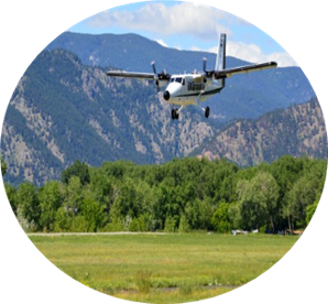
Figure 1:  NEON-AOP: NIWO, RMNP, image from Neon Science

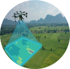
Figure 2: MicaSense Red edge-MX dual  camera data, image from Sky Lark

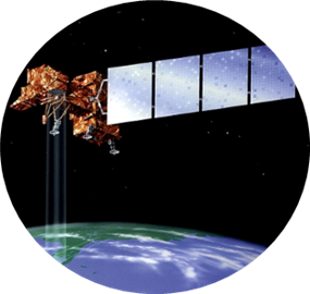
Figure 3: Landsat, image from Earth ESA

2.    Datasets
Our project leverages hyperspectral NEON-AOP data from two sites - the Rocky Mountains National Park (RMNP) and the Niwot Ridge Mountain Research Station (NIWO). The MicaSense Red-edge camera data aids in drone imagery. Central to our mission is a cross-sensor calibration Python tool designed to upscale PFTs fractional canopy cover from high-spatial-resolution sensors (NEON-AOP imaging spectroscopy data and MicaSense drone-based data) to moderate-resolution space-borne sensors like Landsat observations.
 

3.    Workflow Overview

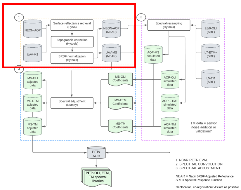
Figure 4: Workflow

For cross sensor calibration, the Macrosystems project's workflow begins with corrections on the NEON-AOP and Drone data as in Figure 4. Through the integration of two correction techniques – the Sun Canopy Sensor Correction and the Sun Canopy Sensor + C Correction (Fang, 2020), we derive optimum results using the latter for drone topography. This then paves the way for the FlexBRDF correction (Queally, 2022). A thorough examination of four combinations of geometric and volume kernels (li-dense, Ross-dense, li-sparse, Ross-sparse) helps in deducing the most consistent corrections across diverse landscapes, primarily targeting the reduction of the across-track brightness effect.
 

4.    Deep Dive into Topographic Correction:
4.1) Why is it significant?
Topographic Correction is important to compensate the influence of terrain variations on the reflectance values of the objects on the Earth`s surface as observed from satellite or sensors. The Earth's topography, or the variation in elevation across the landscape as shown in (Figure 5 and 6), affects how sunlight interacts with the surface, lading to variations in the observed reflectance values. 
 

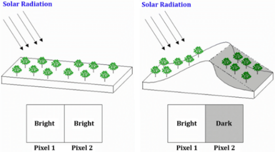
Figure 5: Effect of topography on reflectance, image from (Fang, 2020)

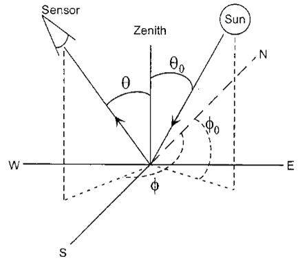
Figure 6: Sun and Sensor angles, image from (Fang, 2020)

4.2)    Methods Employed:

4.2.1)    Sun Canopy Sensor Calibration (SCS): This Normalizes illuminated canopy data. The SCS correction is equivalent to projecting the sunlit canopy from the sloped surface to the horizontal, in the direction of illumination (Queally, 2022). 

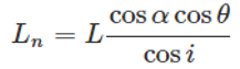
Where, L is the reflectance. cos i  is illumination, α is slope and θ is solar zenith angles.
cos i  is calculated (Ghasemi, 2011): 

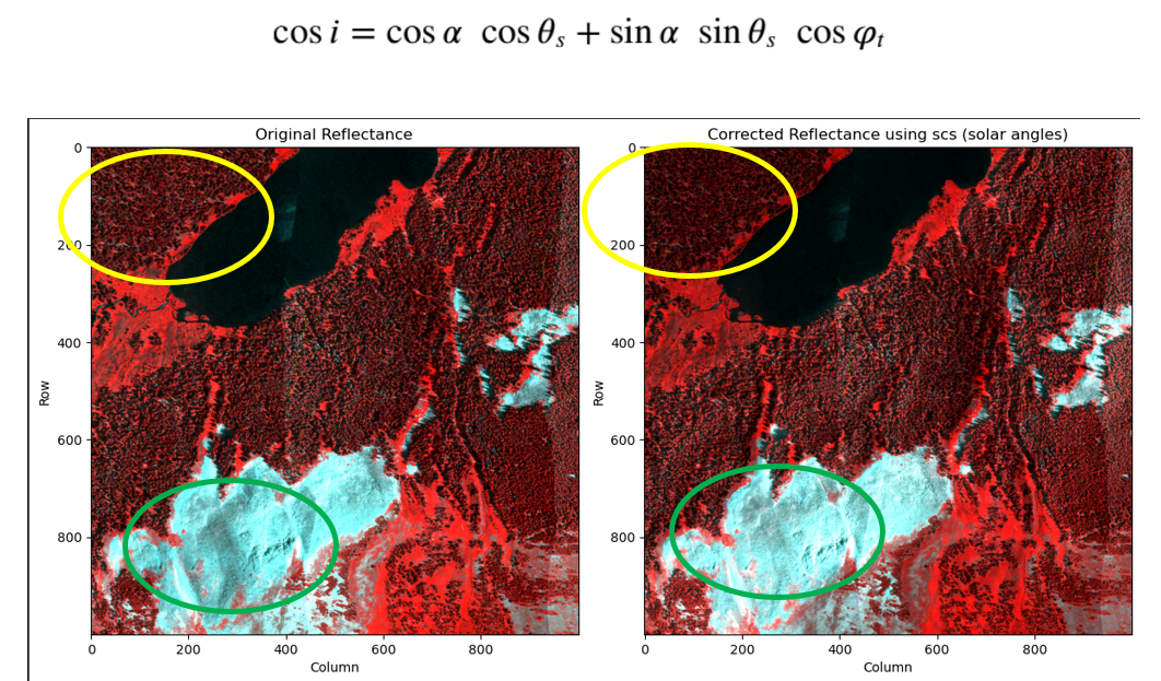
Figure 7: Before and After topographic correction of Band 93 of NIWO site using SCS Correction
Before and after topographic correction we can see that brighter region has become darker and shadier region has become brighter from figure 7.

4.2.2)    Sun Canopy Sensor + C Correction (SCS+C): The SCS + C correction combines the C-correction, which assumes consistent geometry of terrain and trees, with normalized SCS geometry. Topography-induced brightness difference is corrected for each pixel as a function of its slope, solar zenith angle, and relative azimuth angle between the sun and terrain (Queally, 2022).

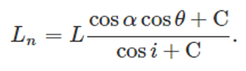
Where C is regression coefficients of reflectance and illumination.

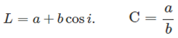
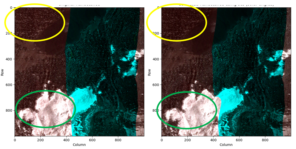
 Figure 8: Before and After topographic correction of Band 93 of NIWO site using SCS + C Correction

4.3)    Topographic Correction of Drone data:
For drone data, which comprises 10 bands, (Claverie, 2018) the SCS+C correction method is implemented. Preliminary steps involve calculating the aspect, slope, and sun angles of the drone data with the help of the Digital Terrain Model (DTM) and ephemeris library.
 

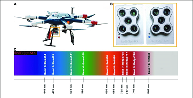
Figure 9: RedEdge-MX dual camera system, image from  (Roman)

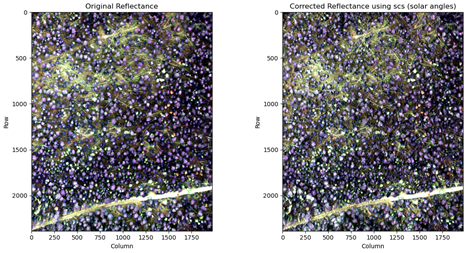
Figure 10: Before and After topographic correction of NIR band of Drone Data using SCS + C Correction

5)  Bidirectional Reflectance Distribution Function (BRDF) Correction:

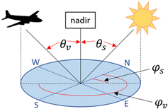
Figure 11 The bidirectional reflectance distribution function is a function of view zenith angle (θv), solar zenith angle (θs), and relative azimuth angle between sun and sensor (φ = φs−φv), image from (Qian)

BRDF correction (Kizel, An unmixing-based BRDF correction in spectral remote sensing data, 2023) is parameterized on the angles of incoming solar light and outgoing sensor light. The potential for BRDF effects stems from variances in how surfaces appear (either sunlit or shaded),(figure 11) influenced by different illumination angles.

FlexBRDF:
It stands out by correcting adjacent flight lines (Queally, 2022), reflecting on the combined reflectance characteristics across all flight lines within a defined area captured on the same day. Harnessing the RossLi kernels, a semi-empirical approach, the tool models the BRDF of surfaces. Our mission is to evaluate four kernel combinations (Ross sparse, Ross Dense, Li sparse and Li Dense) to determine the most consistent correction methods for our vast and varied landscapes

6) Ongoing Work and the Road Ahead:
As of now, our focus remains on the Bidirectional Reflectance Distribution Function (BRDF) Correction. The complexity and depth of the BRDF correction process ensure the validity and reliability of our results. We're diving deep into the nuances of this process, ensuring each aspect is addressed with precision. Following the completion of the BRDF correction, our next steps are clear. We will transition into resampling to the Landsat series band passes and scale the PFTs and data to be analysed across space and time (Claverie, 2018). 
The potential for this open-source sensor cross-calibration tool is expansive. Not only can it scale high-resolution plant spectra to new multispectral and hyperspectral satellite imagery, but its applicability also spans across various ecosystems. This tool promises to revolutionize PFTs disturbance and resilience mapping on a global scale.
GitHub link: https://github.com/earthlab/cross-sensor-cal/tree/janushi-main

6) References:

• Claverie, M. (2018). The Harmonized Landsat and Sentinel-2 surface reflectance data set. Remote Sensing of Environment.
• Fang, Y. (2020). Comparision of Eight Topographic Correction. IOP Conference Series: Earth and Environmental Science.
• Ghasemi, N. (2011). Assessment of different topographic correction. International Journal of Digital Earth.
• Kizel, F. (2023). An unmixing-based BRDF correction in spectral remote sensing data. ScienceDirect.
• Kizel, F. (2023). An unmixing-based BRDF correction in spectral remote sensing data. Science Direct.
• Qian, Y. (n.d.). Assessment of BRDF Impact on VIIRS DNB from Observed Top-of-Atmosphere Reflectance over Dome C in Nighttime. Remote Sensing.
• Queally, N. (2022). FlexBRDF: A Flexible BRDF Correction for Grouped Processing of Airborne Imaging Spectroscopy Flightlines. JGR Biogeosciences.
• Richter, R. (2009). Comparison of Topographic Correction Methods. MDPI.
• Roman, A. (n.d.). Using UAV-Mounted Multispectral camera. Frontier in Marine Science.
• Yao, M. (2022). A comprehensive evaluation method for topographic correction model of remote sensing image based on entropy weight method. Open GeoSciences.
• Ye, Z. (2022). FlexBRDF: A Flexible BRDF Correction for Grouped Processing of Airborne Imaging Spectroscopy Flightlines. Geophysical research and biogeosciences.
• Yin, H. (April 2022). Integrated topographic corrections improve forest mapping using Landsat imagery. ELSEVIER.